
Over 65,000 model configurations evaluated. Nine campaigns closed with a written verdict. One validated candidate. This is what actually survives when you subject machine learning trading models to the same rigour you would demand of a drug trial — with real numbers, including the ones we don’t like.
Most content about AI trading models shows you a spectacular equity curve and hides the process. This page does the opposite: the full validation pipeline, the traps we fell into, the campaigns we closed in the red — and results presented at their true size, which is modest. If you want an article confirming that a neural network can predict the price of bitcoin, this is not it. If you want to know what a serious quantitative process looks like from the inside, you are in the right place — because nobody else in this niche will show it to you.
Everything below comes from our own lab: XGBoost (gradient boosting) and LSTM models trained on BTCUSD and the S&P 500 index, hourly and daily data from 2018 onwards, real transaction costs inside every backtest, and a five-stage validation tunnel that every candidate must pass in full before touching an account — paper trading first, live capital only if it survives that.
Does machine learning work for trading? The short answer and the long one
The question does machine learning work for trading has a short answer almost nobody selling you something will give: almost never — and that is exactly why methodology matters more than the model.
Our lab’s numbers: on the order of 65,000 optimization trials (each one a complete model configuration, trained and evaluated) across more than a dozen campaigns on BTCUSD, SPX500, XAUUSD and volatility derivatives. Out of all that compute came exactly two things: one system in production and one validated candidate on the S&P 500 about to enter paper trading. Everything else — nine bitcoin timeframes, three gold campaigns, five architectures on crypto candles — ended in an archive with a written closing verdict.
That ratio — 65,000 tried, one kept — is not a confession. It is the product. Machine learning always finds patterns; those patterns existing outside the training sample is the exception. A validation pipeline is not there to find winners: it is there to kill, quickly and cheaply, the thousands of impostors an optimizer produces — so that whatever little survives deserves trust.
Feature engineering for crypto trading: what goes into the model and why
Feature engineering in crypto trading — and in index trading — is where the game is won or lost before anything gets trained. After testing hundreds of features, our experience fits into three principles and a graveyard.
Few features, from the same family of information. Our validated S&P 500 candidate uses exactly 8 inputs; the best model of the entire bitcoin campaign used 7. In both cases the search was free to use more and converged on fewer by itself. We can reveal the S&P 500 composition because individual features are not the secret (the exact configuration and trained model are): distances to structural swing highs over 12 and 24 bars, distance to session open, realized volatility ratio, positive realized semivariance, realized jump skewness, an ATR ratio and the normalized upper wick of the candle. Nothing exotic — price structure, realized volatility and candle microstructure, all normalized to stay comparable across regimes.
Feature importance does not tell you what is safe to remove. We learned the hard way that XGBoost’s importance ranking is useless for pruning: low-importance features turned out to be load-bearing (removing them sank the out-of-sample), and dominant features turned out to be redundant. The only valid test is ablation measured on validation — one feature at a time, one change per experiment.
Calendar features are overfitting magnets. The sine/cosine encoding of hour-of-day is the most dangerous feature we have ever handled: in XGBoost it once captured 60% of a model’s importance — a model whose out-of-sample then collapsed. Trees use it to memorize episodes (“Tuesdays at 3pm in 2021, X happened”) instead of generalizing. We removed it from every gradient boosting model and only keep it, under watch, as a sequential input to LSTMs.
The graveyard. These features died with evidence against them and are not coming back: MACD, Hurst exponent, wick skewness, normalized ADX, Bollinger-band position, simple return z-scores, distance to the 50-period EMA, the Corwin-Schultz spread estimator, and the variance risk premium as a standalone signal. Every one of them looked promising in some grid; none survived serious validation. We publish the list because half the content out there on xgboost trading strategy is built on exactly these.
In-sample vs out-of-sample trading: the partition architecture that decides everything
The in-sample vs out-of-sample distinction looks trivial — train here, evaluate there — and yet it is where most projects die, for a subtle reason: having a test block is not enough. You have to protect it from yourself.
Our architecture uses four chronological blocks with purge gaps between them, so one partition’s labeling never sees the next partition’s prices: training (~54%), an early internal validation, an external validation (~20%) and a final test (~20%) that plays no role in any search decision. The optimizer maximizes the validation result; the test is computed and stored, but no configuration is ever selected by its test score.
Why all the theater? Because failure has a signature we have now seen dozens of times. In our latest S&P 500 campaign, the top-ranked trial by validation out of 5,880 showed runaway memorization and a stellar validation of 4.89… which became 0.58 on test. The top trial of a ranking is almost never a system: it is the winner of an overfitting lottery. We discard it by rule, not by intuition. The inverse trap is just as lethal — scanning the test column and “discovering” trials that look brilliant there is test-picking: it turns the test into just another validation and leaves you with no virgin data at all. House rule, no exceptions: selection is always by validation.
You can see this decay measured on real data on our home page record: the full backtest of our daily bitcoin model, with the in-sample region explicitly hatched and the out-of-sample period plotted separately. In-sample it compounds near +47% a year; out-of-sample, near +7%. The model is roughly eight times its out-of-sample self inside the training set — and publishing both numbers side by side is precisely the point. Any strategy that shows you only one of them is showing you the wrong one.
Walk forward optimization in trading: the tribunal every candidate must face
Walk forward optimization is the stage that separates our methodology from a backtest with extras — and where walk forward analysis on bitcoin taught us the most expensive lesson of the project.
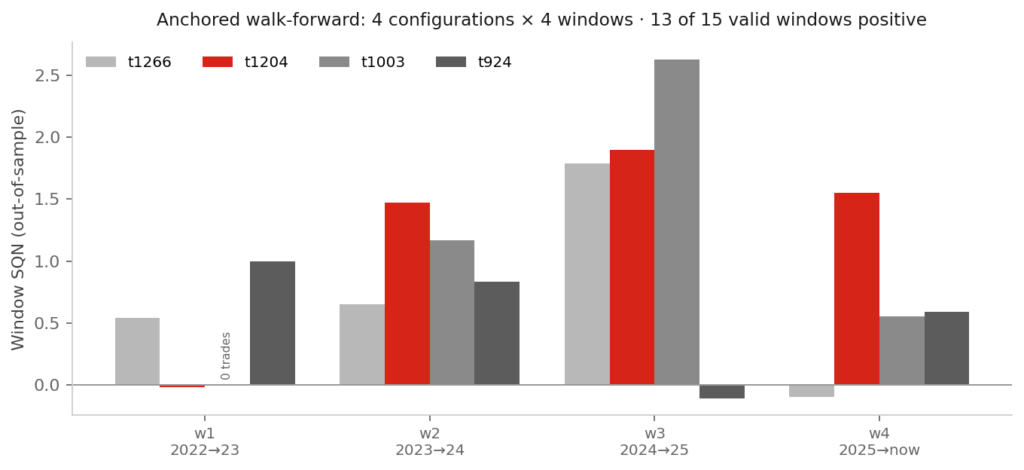
The design: contiguous, anchored test windows. The model is retrained from 2018 up to the eve of each window and evaluated on the following block, repeatedly, covering 2022 through today. Each window is a simulated deployment — what would have happened had we frozen the model on that date? And the most important part is not the design but the pre-registration: pass criteria are written down before anything runs. In our case: at least 3 of 4 conclusive windows positive, an aggregate SQN ≥ 1.0, and veto power for the most recent window — if the current regime is negative, it does not matter how pretty the history looks.
The success case, on the S&P 500: not one trial but a cluster of four neighbouring configurations sharing the same 8 features with slightly different hyperparameters. All four passed the walk-forward independently: 13 of 15 valid windows positive, aggregate SQNs between 1.04 and 1.80. Four variants of the same region of parameter space surviving independently is a class of evidence no single trial can provide.
The instructive case, on bitcoin: our best daily BTCUSD candidate reached the walk-forward with excellent headline metrics. The tribunal ruled otherwise — the only virgin window with a sufficient sample delivered an SQN of +0.52, positive but insufficient, and all of the candidate’s apparent strength lived exactly in the partition over which three search passes totaling ~13,000 trials had been run. An echo of the mining, not signal. It hurts far more to archive a candidate with +90% cumulative on its curve than a mediocre one — which is exactly why the criteria are written before seeing the results.
That daily bitcoin model is the one whose complete record this site publishes — and its next tribunal is running right now, in public. Every trade it takes is posted to Telegram the moment it happens and tracked independently by FXBlue, against criteria fixed in advance. The backtest said “promising but unproven”; instead of arguing with that verdict, we are settling it the only way it can be settled — forward, on data nobody has seen, where you can watch. Most sites show you a curve and ask for trust. This one shows you the validation phase itself, live.
How to avoid backtest overfitting: four defenses that actually work
If one question sums up this craft it is how to avoid backtest overfitting, and our answer after 65,000 trials is that you do not avoid it with one technique. You avoid it in layers.
1 · Hunt plateaus, not peaks
An isolated maximum in parameter space is almost always an artifact; a region where many neighbouring configurations work is a property of the market. Our gate requires at least 60% of dense neighbours to show positive validation. The S&P 500 cluster delivered 54 of 61 positive neighbours (89%).
2 · Reproduce before you publish
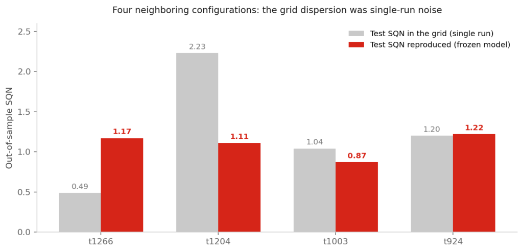
A grid cell once read test SQN 2.23; the rebuilt frozen model read 1.11. The dispersion between nearly identical configurations was single-run noise, and 2.23 was its lucky end. The honest figure is the reproducible one — and that is the only number that reaches a system sheet.
3 · Monte Carlo over the sequence
A result cannot depend on those trades in that order. We resample the out-of-sample walk-forward trades, dropping 10% at random, ten thousand times. For the validated candidate, the 5th percentile stayed at +20.7 points and not one of 10,000 iterations ended negative.
4 · Cost stress
We closed an entire volatility campaign upon discovering the real spread was 34× the modeled one — an error no walk-forward detects, because it contaminates every partition equally. Every candidate must now survive a tripling of its transaction costs.
LSTM vs XGBoost for time series: what we actually measured
The LSTM vs XGBoost time series debate is usually framed as a race. Our data says something less comfortable and more useful.
On the S&P 500, the LSTM added no value over gradient boosting — and we measured it properly. The architecture was hybrid: an LSTM with attention processes feature sequences and condenses its reading into two probabilities that feed XGBoost as extra inputs. After stabilizing the experiment, the best hybrid reached a validation objective of 1.79 against 3.30 for XGBoost alone. Not for lack of trying: hundreds of trials with iterable windows, sizes and input sets.
That “after stabilizing” hides a lesson worth the price of admission on its own: LSTM training is not deterministic, and the variance across seeds was large enough to dominate any comparison — two identical trainings could differ by more than two different configurations. The fix that worked was ensembling no fewer than 6 members with different seeds. Any result from an LSTM trained once is, literally, a lottery ticket — and if an article about bitcoin price prediction with machine learning does not mention this problem, its authors have not trained the model enough times to meet it.
From a mass analysis of 829 trials with iterable input selection came concrete numbers: the distance to the 24-bar structural high appeared in 92% of top-decile trials (against a 46% baseline), and the distance to session open in 71% — the two most robust sequential inputs we have ever measured. Our current position: XGBoost as the backbone, for its deterministic reproducibility and robustness on small data; the LSTM only as a sequential feature generator, only in ensembles, and only if it proves in validation that it adds signal.
What we discarded: the campaign graveyard, with numbers
No methodology page is credible without this section — and no competitor will write it, which is why it is here.
Directional bitcoin: 9 timeframe configurations, ~30,000 trials, zero unconditional survivors. We swept from 10-minute to daily candles. Fast timeframes proved non-evaluable with standard triple-barrier labeling until we discovered that barriers must scale with the square root of the horizon. With the instrument corrected, the answer came back clean, and it was negative across the 2-to-12-hour band. On the daily timeframe, the best candidate’s story is told above.
Gold: three independent campaigns, no deployable edge. XAUUSD produces attractive backtests with ease; none survived temporal cross-validation. Volatility derivatives: closed on costs — the campaign was mathematically unviable at the instrument’s real spread. Five architectures on crypto candles: all test-negative, from pattern classifiers to sequential hybrids.
The joint reading matters more than each closure: the machinery that validates a candidate is the same machinery that rejected everything above. A pipeline that only produces approvals is validating nothing. The rejection rate is the approval’s certificate of authenticity — and ours has archived over 60,000 configurations to keep one.
What a verified trading track record actually means
It pays to be exact with words here, because verified bitcoin trading track record is one of the most manipulated searches in this industry. A backtest is not a track record. A walk-forward is not one either. A verified track record is a sequence of trades executed in a real or simulated account, with timestamps preceding the outcomes, against success and kill criteria written before the first trade.
That definition is the standard this site holds itself to. Kill criteria are pre-registered — automatic pause if net P&L is ≤ 0 after a fixed number of trades or months, immediate pause at a drawdown ceiling the backtest never touched — and every trade is published the moment it happens, timestamped on Telegram and read independently by FXBlue. When the record is long enough to mean something, it will mean something precisely because the criteria were public before it existed.
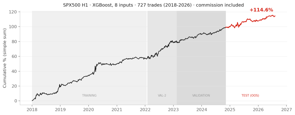
And the limits are part of the result. Validated edges in this business are modest: real-system SQNs live near 1.0-1.8, not 3. Performance decays — our candidate’s per-trade edge has drifted from +0.20% to +0.08% across seven years, still positive, slope documented. Edges erode; a system without a retirement plan is a system without a plan. If someone shows you a curve without decay, without a rejection archive and without pre-registered kill criteria, you are not looking at research. You are looking at marketing.
Conclusions
Three sentences carry the essentials. Machine learning applied to trading works on the rare occasions it works, and only a pipeline designed to reject can identify those occasions — selection exclusively by validation, anchored walk-forward with pre-registered criteria, plateaus instead of peaks, reproduction before publication, Monte Carlo over the sequence, cost stress. XGBoost beats LSTMs on tabular price data, and any LSTM result without a seed ensemble is noise with good posture. And the metric that truly predicts the quality of a methodology is not its best curve but its rejection rate.
Everything this lab publishes — the live trades, the backtest with its in-sample region marked, the archive of what failed — exists so you can audit that claim instead of trusting it.
This page summarizes methodology and aggregate results. Full configurations, trained models and exact execution parameters are not published. All figures include real transaction costs and constitute neither investment advice nor a guarantee of future performance. See the full risk disclosure.